
EM 1110-2-1100 (Part II)
30 Apr 02
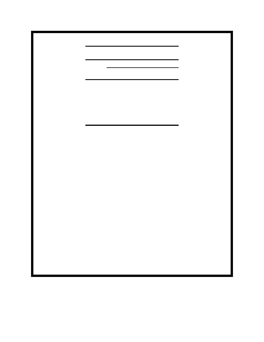
Example Problem II-8-2 (Continued)
Table II-8-20
Design Significant Wave Heights at Jetty Head
Jetty Design
Toe Design
Tr
Hsjetty
Hstoe
(yr)
(cm)
(cm)
2
732
612
5
753
622
10
768
628
25
789
637
50
804
644
100
819
650
If a design life longer than 25 years were needed, values of Hsjetty approaching the maximum based on maximum
tide level might need to be considered. This maximum represents an increase of about 1 m in Hsjetty at any selected
return period, which would significantly influence jetty design. There is some chance of the maximum occurring
even in a 25-year design life. That possibility should be considered if risks are analyzed. Also it should be
recognized that the great hydrodynamic energy associated with design events can significantly change nearshore
bottom elevations. Storm-induced scour could subject the jetty to increased wave heights, possibly approaching
the maximum during shoaling at the jetty head. This effect should also be considered in risk analysis.
Design wave heights - jetty toe. Past physical model studies of some jetty cross sections have shown that waves
attacking at water levels of around MLLW are most likely to cause damage to the underwater portion of the
structure, including the toe. Similar behavior is assumed in this example. Since this jetty is in a high wave energy
environment with fairly large tide range, it is worthwhile to estimate extreme wave heights at MLLW. The lower
wave heights (because of reduced depth) can be assessed relative to the lower stability of underwater armor units
(due to less precise placement).
Values of H0' and H0'/L0 for each of the observed events (Table II-8-13) are used with a water depth of 10 m
(corresponding to MLLW at the jetty head), and bottom slope of 1/100 to estimate a significant wave height for
toe design Hstoe for each event (illustrated in Table II-8-21 for one event). These 33 values of Hstoe were subjected
to extremal analysis (Figure II-8-30). The shallow depth greatly limits wave heights, and Hstoe values are confined
to a very narrow range between 5.8 m and 6.5 m. The Weibull distribution function with k = 2.0, which best
simulates the shape of a capped distribution function (Figure II-8-3), provides the best fit. Hstoe values for design
are summarized in Table II-8-20.
Example Problem II-8-2 (Sheet 17 of 21)
Hydrodynamic Analysis and Design Conditions
II-8-51

 Previous Page
